\(\text{Model 2 molecules}\)
[4]:
import pyvcham
import numpy as np
import matplotlib.pyplot as plt
import json
[5]:
"""
This is an example of a VC model of a simple 1D system which consists of 2 electronic states.
The model is build from a database of a real system, precisely the full dimensional model of FCHO molecule.
We just take one of the coordinates and build a 1D model from it.
"""
[5]:
'\nThis is an example of a VC model of a simple 1D system which consists of 2 electronic states.\nThe model is build from a database of a real system, precisely the full dimensional model of FCHO molecule.\nWe just take one of the coordinates and build a 1D model from it.\n'
[10]:
# Create a database in eV with all the abinitio data
step = 10
q = np.arange(-100, 100 + step, step)
nmodes = 6
data_gs = []
data_val = []
data_carbon = []
all_q = []

path  = "abinitio_data/"
min_scf = np.array(json.load(open(path + "geo_v1_00.json"))["ground_state"]["scf_energy"])
min_mp2 = np.array(json.load(open(path + "geo_v1_00.json"))["ground_state"]["mp2_correction"])
min_mp3 = np.array(json.load(open(path + "geo_v1_00.json"))["ground_state"]["mp3_correction"])
min_gs = min_scf + min_mp2 + min_mp3

for mode in range(1, nmodes+1):
    temp_gs = []
    temp_val = []
    temp_carbon = []
    temp_q = []
    for disp in q:
        geo = f"geo_v{mode}_{disp:02d}"
        path2 = f"{path}{geo}.json"
        data = json.load(open(path2))
        scf = data["ground_state"]["scf_energy"]
        mp2 = data["ground_state"]["mp2_correction"]
        mp3 = data["ground_state"]["mp3_correction"]
        gs_energy = scf + mp2 + mp3
        val = data["valence"]["excitation_energy"]
        carbon = data["carbon_core"]["excitation_energy"]

        # gs_energy should be below a threshold
        if gs_energy - min_gs < 0.4:
            temp_gs.append(gs_energy)
            temp_val.append(val)
            temp_carbon.append(carbon)
            temp_q.append(disp)

    temp_gs = np.array(temp_gs)
    temp_val = np.array(temp_val)
    temp_carbon = np.array(temp_carbon)
    temp_q = np.array(temp_q)

    temp_val = np.transpose(temp_val, (1,0))
    temp_val = ((temp_val + temp_gs) - min_gs)* pyvcham.constants.AU_TO_EV

    temp_carbon = np.transpose(temp_carbon, (1,0))
    temp_carbon = ((temp_carbon + temp_gs) - min_gs)* pyvcham.constants.AU_TO_EV
    temp_gs = (temp_gs - min_gs)* pyvcham.constants.AU_TO_EV


    all_q.append(temp_q)
    data_gs.append(temp_gs)
    data_val.append(temp_val)
    data_carbon.append(temp_carbon)
[11]:
data_pyvcham = []
q_pyvcham = []
for mode in range(nmodes):
    data_mode = []
    data_mode.append(data_gs[mode])
    for state in range(5):
        data_mode.append(data_val[mode][state])
    q_pyvcham.append(np.array(all_q[mode])/10)
    data_pyvcham.append(np.array(data_mode))

data_pyvcham[2][1] = data_pyvcham[2][1] + 0.3 *q_pyvcham[2]
[13]:
# Creating the VC system object
vib_freq = np.array([1113.0039]) * pyvcham.constants.CM1_TO_AU * pyvcham.constants.AU_TO_EV  # in eV

# Guess diabatic function for each mode
diab_f_each_mode = ["morse"]
diab_funct_mode = [[mode] * 2 for mode in diab_f_each_mode]

system = pyvcham.VCSystem(
    vc_type= "linear",
    units="eV",
    number_normal_modes=1,
    number_states=2,         # GS + 1 excited state
    coupling_with_gs=True,
    symmetry_point_group="Cs",
    symmetry_states = ["Ap", "App"],
    symmetry_modes = [ "Ap"],
    vib_freq= vib_freq,  # to eV
    diab_funct= diab_funct_mode,
    displacement_vector= [q_pyvcham[2]],
    database_abinitio=[data_pyvcham[2][:2]],

)
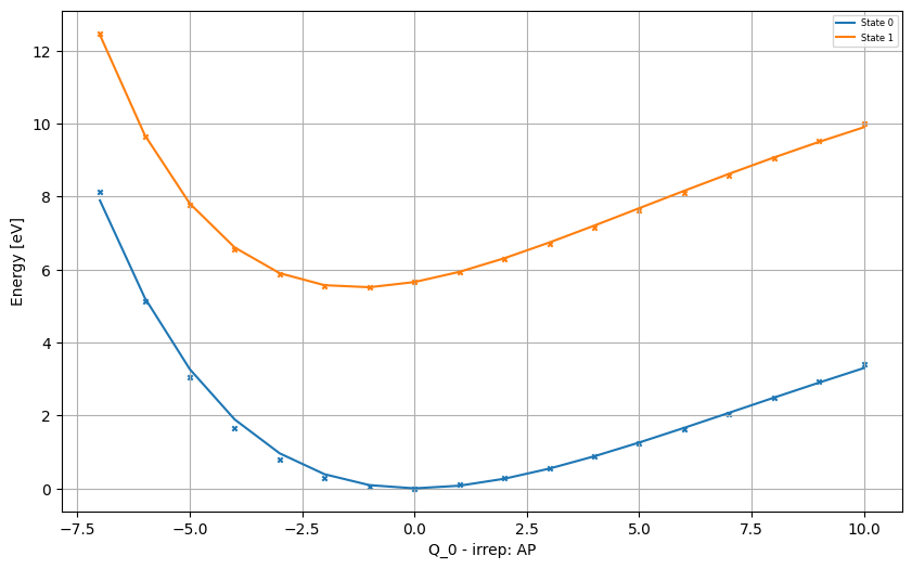
2025-11-27 10:23:46,994 [INFO] pyvcham.vcham_system: Computed vertical energy shifts: [1.08275176e-11 5.65868614e+00]
[15]:
# Setting up the model parameters

for mode in range(system.number_normal_modes):
    model = pyvcham.LVCHam(normal_mode=mode,VCSystem=system,nepochs=10000)
    model.initialize_params()
    model.initialize_loss_function()
    model.optimize()
2025-11-27 10:24:06,478 [INFO] pyvcham.lvc:

----- Initializing LVC Hamiltonian Builder -----
2025-11-27 10:24:06,479 [INFO] pyvcham.lvc: Normal mode: 0
2025-11-27 10:24:06,483 [INFO] pyvcham.lvc: JT off-diagonal pairs: []
2025-11-27 10:24:06,483 [INFO] pyvcham.lvc: n_var_list (non-JT): [3, 3]
2025-11-27 10:24:06,485 [INFO] pyvcham.lvc: Total parameters to optimize: 6
2025-11-27 10:24:06,485 [INFO] pyvcham.lvc: Optimizing mode 0...
2025-11-27 10:24:06,777 [INFO] pyvcham.lvc: Step 0, Loss: 437.718567
2025-11-27 10:24:06,827 [INFO] pyvcham.lvc: Step 100, Loss: 104.557541
2025-11-27 10:24:06,862 [INFO] pyvcham.lvc: Step 200, Loss: 23.480787
2025-11-27 10:24:06,897 [INFO] pyvcham.lvc: Step 300, Loss: 3.830597
2025-11-27 10:24:06,931 [INFO] pyvcham.lvc: Step 400, Loss: 0.232904
2025-11-27 10:24:06,965 [INFO] pyvcham.lvc: Step 500, Loss: 0.193453
2025-11-27 10:24:07,000 [INFO] pyvcham.lvc: Step 600, Loss: 0.163423
2025-11-27 10:24:07,037 [INFO] pyvcham.lvc: Step 700, Loss: 0.138704
2025-11-27 10:24:07,078 [INFO] pyvcham.lvc: Step 800, Loss: 0.117632
2025-11-27 10:24:07,118 [INFO] pyvcham.lvc: Step 900, Loss: 0.099614
2025-11-27 10:24:07,158 [INFO] pyvcham.lvc: Step 1000, Loss: 0.084305
2025-11-27 10:24:07,198 [INFO] pyvcham.lvc: Step 1100, Loss: 0.071582
2025-11-27 10:24:07,236 [INFO] pyvcham.lvc: Step 1200, Loss: 0.061147
2025-11-27 10:24:07,270 [INFO] pyvcham.lvc: Step 1300, Loss: 0.052766
2025-11-27 10:24:07,305 [INFO] pyvcham.lvc: Step 1400, Loss: 0.046205
2025-11-27 10:24:07,340 [INFO] pyvcham.lvc: Step 1500, Loss: 0.041074
2025-11-27 10:24:07,375 [INFO] pyvcham.lvc: Step 1600, Loss: 0.037043
2025-11-27 10:24:07,409 [INFO] pyvcham.lvc: Step 1700, Loss: 0.033839
2025-11-27 10:24:07,443 [INFO] pyvcham.lvc: Step 1800, Loss: 0.031243
2025-11-27 10:24:07,478 [INFO] pyvcham.lvc: Step 1900, Loss: 0.029083
2025-11-27 10:24:07,514 [INFO] pyvcham.lvc: Step 2000, Loss: 0.027230
2025-11-27 10:24:07,553 [INFO] pyvcham.lvc: Step 2100, Loss: 0.025596
2025-11-27 10:24:07,592 [INFO] pyvcham.lvc: Step 2200, Loss: 0.024118
2025-11-27 10:24:07,629 [INFO] pyvcham.lvc: Step 2300, Loss: 0.022757
2025-11-27 10:24:07,668 [INFO] pyvcham.lvc: Step 2400, Loss: 0.021490
2025-11-27 10:24:07,706 [INFO] pyvcham.lvc: Step 2500, Loss: 0.020299
2025-11-27 10:24:07,742 [INFO] pyvcham.lvc: Step 2600, Loss: 0.019177
2025-11-27 10:24:07,776 [INFO] pyvcham.lvc: Step 2700, Loss: 0.018118
2025-11-27 10:24:07,811 [INFO] pyvcham.lvc: Step 2800, Loss: 0.017116
2025-11-27 10:24:07,875 [INFO] pyvcham.lvc: Step 2900, Loss: 0.016170
2025-11-27 10:24:07,910 [INFO] pyvcham.lvc: Step 3000, Loss: 0.015277
2025-11-27 10:24:07,945 [INFO] pyvcham.lvc: Step 3100, Loss: 0.014434
2025-11-27 10:24:07,979 [INFO] pyvcham.lvc: Step 3200, Loss: 0.013638
2025-11-27 10:24:08,014 [INFO] pyvcham.lvc: Step 3300, Loss: 0.012889
2025-11-27 10:24:08,049 [INFO] pyvcham.lvc: Step 3400, Loss: 0.012183
2025-11-27 10:24:08,083 [INFO] pyvcham.lvc: Step 3500, Loss: 0.011520
2025-11-27 10:24:08,117 [INFO] pyvcham.lvc: Step 3600, Loss: 0.010896
2025-11-27 10:24:08,152 [INFO] pyvcham.lvc: Step 3700, Loss: 0.010310
2025-11-27 10:24:08,186 [INFO] pyvcham.lvc: Step 3800, Loss: 0.009761
2025-11-27 10:24:08,220 [INFO] pyvcham.lvc: Step 3900, Loss: 0.009247
2025-11-27 10:24:08,254 [INFO] pyvcham.lvc: Step 4000, Loss: 0.008765
2025-11-27 10:24:08,288 [INFO] pyvcham.lvc: Step 4100, Loss: 0.008316
2025-11-27 10:24:08,322 [INFO] pyvcham.lvc: Step 4200, Loss: 0.007896
2025-11-27 10:24:08,357 [INFO] pyvcham.lvc: Step 4300, Loss: 0.007505
2025-11-27 10:24:08,391 [INFO] pyvcham.lvc: Step 4400, Loss: 0.007142
2025-11-27 10:24:08,425 [INFO] pyvcham.lvc: Step 4500, Loss: 0.006804
2025-11-27 10:24:08,460 [INFO] pyvcham.lvc: Step 4600, Loss: 0.006493
2025-11-27 10:24:08,494 [INFO] pyvcham.lvc: Step 4700, Loss: 0.006201
2025-11-27 10:24:08,529 [INFO] pyvcham.lvc: Step 4800, Loss: 0.005938
2025-11-27 10:24:08,563 [INFO] pyvcham.lvc: Step 4900, Loss: 0.005688
2025-11-27 10:24:08,597 [INFO] pyvcham.lvc: Step 5000, Loss: 0.005464
2025-11-27 10:24:08,631 [INFO] pyvcham.lvc: Step 5100, Loss: 0.005253
2025-11-27 10:24:08,665 [INFO] pyvcham.lvc: Step 5200, Loss: 0.005071
2025-11-27 10:24:08,699 [INFO] pyvcham.lvc: Step 5300, Loss: 0.004889
2025-11-27 10:24:08,732 [INFO] pyvcham.lvc: Step 5400, Loss: 0.004747
2025-11-27 10:24:08,767 [INFO] pyvcham.lvc: Step 5500, Loss: 0.004588
2025-11-27 10:24:08,800 [INFO] pyvcham.lvc: Step 5600, Loss: 0.004463
2025-11-27 10:24:08,835 [INFO] pyvcham.lvc: Step 5700, Loss: 0.004341
2025-11-27 10:24:08,870 [INFO] pyvcham.lvc: Step 5800, Loss: 0.004237
2025-11-27 10:24:08,905 [INFO] pyvcham.lvc: Step 5900, Loss: 0.004142
2025-11-27 10:24:08,941 [INFO] pyvcham.lvc: Step 6000, Loss: 0.004058
2025-11-27 10:24:08,979 [INFO] pyvcham.lvc: Step 6100, Loss: 0.003984
2025-11-27 10:24:09,014 [INFO] pyvcham.lvc: Step 6200, Loss: 0.003926
2025-11-27 10:24:09,047 [INFO] pyvcham.lvc: Step 6300, Loss: 0.003860
2025-11-27 10:24:09,081 [INFO] pyvcham.lvc: Step 6400, Loss: 0.003810
2025-11-27 10:24:09,115 [INFO] pyvcham.lvc: Step 6500, Loss: 0.003764
2025-11-27 10:24:09,149 [INFO] pyvcham.lvc: Step 6600, Loss: 0.003734
2025-11-27 10:24:09,182 [INFO] pyvcham.lvc: Step 6700, Loss: 0.003692
2025-11-27 10:24:09,216 [INFO] pyvcham.lvc: Step 6800, Loss: 0.003663
2025-11-27 10:24:09,249 [INFO] pyvcham.lvc: Step 6900, Loss: 0.003639
2025-11-27 10:24:09,283 [INFO] pyvcham.lvc: Step 7000, Loss: 0.003627
2025-11-27 10:24:09,315 [INFO] pyvcham.lvc: Step 7100, Loss: 0.003600
2025-11-27 10:24:09,349 [INFO] pyvcham.lvc: Step 7200, Loss: 0.003588
2025-11-27 10:24:09,380 [INFO] pyvcham.lvc: Step 7300, Loss: 0.003573
2025-11-27 10:24:09,413 [INFO] pyvcham.lvc: Step 7400, Loss: 0.003562
2025-11-27 10:24:09,445 [INFO] pyvcham.lvc: Step 7500, Loss: 0.003554
2025-11-27 10:24:09,477 [INFO] pyvcham.lvc: Step 7600, Loss: 0.003547
2025-11-27 10:24:09,509 [INFO] pyvcham.lvc: Step 7700, Loss: 0.003542
2025-11-27 10:24:09,541 [INFO] pyvcham.lvc: Step 7800, Loss: 0.003537
2025-11-27 10:24:09,572 [INFO] pyvcham.lvc: Step 7900, Loss: 0.003537
2025-11-27 10:24:09,602 [INFO] pyvcham.lvc: Step 8000, Loss: 0.003530
2025-11-27 10:24:09,633 [INFO] pyvcham.lvc: Step 8100, Loss: 0.003528
2025-11-27 10:24:09,663 [INFO] pyvcham.lvc: Step 8200, Loss: 0.003526
2025-11-27 10:24:09,693 [INFO] pyvcham.lvc: Step 8300, Loss: 0.003525
2025-11-27 10:24:09,723 [INFO] pyvcham.lvc: Step 8400, Loss: 0.003524
2025-11-27 10:24:09,753 [INFO] pyvcham.lvc: Step 8500, Loss: 0.003534
2025-11-27 10:24:09,783 [INFO] pyvcham.lvc: Step 8600, Loss: 0.003522
2025-11-27 10:24:09,812 [INFO] pyvcham.lvc: Step 8700, Loss: 0.003522
2025-11-27 10:24:09,842 [INFO] pyvcham.lvc: Step 8800, Loss: 0.003521
2025-11-27 10:24:09,872 [INFO] pyvcham.lvc: Step 8900, Loss: 0.003521
2025-11-27 10:24:09,901 [INFO] pyvcham.lvc: Step 9000, Loss: 0.003521
2025-11-27 10:24:09,931 [INFO] pyvcham.lvc: Step 9100, Loss: 0.003521
2025-11-27 10:24:09,961 [INFO] pyvcham.lvc: Step 9200, Loss: 0.003521
2025-11-27 10:24:09,988 [INFO] pyvcham.lvc: Early stopping triggered at step 9290 (no improvement for 150 steps). Best loss: 0.003521
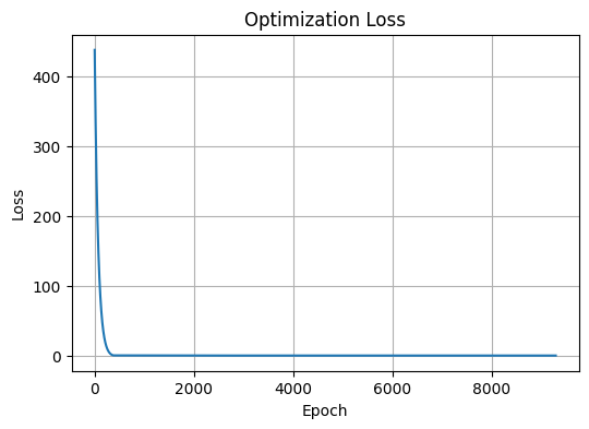
2025-11-27 10:24:10,152 [INFO] pyvcham.lvc: Optimization finished – Final reported loss: 0.003521
2025-11-27 10:24:10,152 [INFO] pyvcham.lvc: Optimization completed in 3.50 seconds.
[16]:
# Defining the geometry of the system
geometry = [("X", [0,0,-0.5]),  # X means Ghost atom
            ("X", [0,0,0.5])]

# Adding the geometry to the system
system.add_geometry(geometry)

# Defining the general data of the system
general_data = {
    "molecule": "diatomic model",
    "calculation_info": "Valence excitation",
}
2025-11-27 10:24:14,040 [INFO] pyvcham.vcham_system: Reference geometry updated.
\(\Sigma^+\) transition
Only the z-component is non-zero for the transition dipole
[17]:
# Defining the dipole matrix
dipole_matrix = np.array([
    [[0, 0, 0], [0, 0, 1]],
    [[0, 0, 1], [0, 0, 0]]
])
# The dipole matrix size should be (number_states, number_states, 3). The last dimension corresponds to the x, y, z components of the dipole moment.
# Adding the dipole matrix to the system
system.add_dipole_matrix(dipole_matrix)

# Saving the system to a JSON file and converting it to MCTDH format
name = "model_sigma_plus"
filename_json = name + ".json"
pyvcham.utils.VCSystem_to_json(system, general_data, filename_json,rewrite=True)
output_file = name + ".op"
pyvcham.utils.json_to_mctdh(filename_json, output_file)
2025-11-27 10:24:16,919 [INFO] pyvcham.vcham_system: Dipole matrix updated.
2025-11-27 10:24:16,922 [INFO] pyvcham.utils: Warning: Overwriting existing file model_sigma_plus.json
2025-11-27 10:24:16,924 [INFO] pyvcham.utils: Data successfully saved to model_sigma_plus.json
2025-11-27 10:24:16,925 [INFO] pyvcham.utils: No interactions found.
2025-11-27 10:24:16,926 [INFO] pyvcham.utils: MCTDH operator file successfully written to: model_sigma_plus.op
[18]:
# Now let us create a supersystem with the model consisting of two identical subsystems.
# The two subsystems will be placed at a distance of 10 Bohr.

r = 10
r_angstrom = r * pyvcham.constants.BOHR_TO_ANGSTROM
print(f"Distance in Angstrom: {r_angstrom}, Distance in Bohr: {r}")


# We have to define the molecules and interactions between them
# Define the two molecules with their interacting states and positions
# The first molecule is at the origin, the second one is at (0, 0, r)
# The two molecules will be parallel to the z-axis, but you can change the rotation angles to make them perpendicular or at any other angle.

mol1 = pyvcham.utils.Molecule(molecule_idx=0, interacting_states=[0,1],CM=np.array([0.0, 0.0, 0.0]), rot_angles=(0.0, 0.0, 0.0))
# mol2 = pyvcham.utils.Molecule(molecule_idx=1, interacting_states=[0,1],CM=np.array([0.0, 0.0, r]), rot_angles=(0.0,0.0,0.0)) # Parallel to the z-axis
mol2 = pyvcham.utils.Molecule(molecule_idx=1, interacting_states=[0,1],CM=np.array([0.0, 0.0, r]), rot_angles=(0.0,0.0,0.0)) # Perpendicular to the z-axis

# Define interactions among molecules
# In this case, we will use the dipole-dipole interaction.
int1 = pyvcham.utils.DipoleInteraction(molecules=[mol1,mol2])

# Save the interaction data to a JSON file
# The infiles are the JSON files of the individual molecules, which we will use to merge them into a single JSON file.
# The outfile is the name of the output JSON file, which will contain the merged data of the two molecules and their interaction.
# The molecules and interactions are passed as lists, so you can add more molecules and interactions if needed.
pyvcham.utils.merge_jsons(infiles=[filename_json, filename_json],
                  outfile="2mol_model_sigma_plus.json",
                  molecules=[mol1, mol2],
                  interactions=[int1],
                  rewrite=True
                  )

pyvcham.utils.json_to_mctdh("2mol_model_sigma_plus.json", "2mol_model_sigma_plus.op")
2025-11-27 10:24:17,569 [INFO] pyvcham.utils: Reading 2 JSON files and merging them.
2025-11-27 10:24:17,572 [INFO] pyvcham.utils:
Molecule 0 new geometry in the fixed lab frame:
[[ 0.   0.  -0.5]
 [ 0.   0.   0.5]]

2025-11-27 10:24:17,573 [INFO] pyvcham.utils:
Molecule 1 new geometry in the fixed lab frame:
[[ 0.   0.  -0.5]
 [ 0.   0.   0.5]]

2025-11-27 10:24:17,574 [INFO] pyvcham.utils: Calculating dipole interaction for pair Molecule0 - Molecule1

2025-11-27 10:24:17,577 [INFO] pyvcham.utils: Warning: Overwriting existing file 2mol_model_sigma_plus.json
2025-11-27 10:24:17,579 [INFO] pyvcham.utils: Data successfully saved to 2mol_model_sigma_plus.json
2025-11-27 10:24:17,581 [INFO] pyvcham.utils: Interactions found!
2025-11-27 10:24:17,582 [INFO] pyvcham.utils: Dipole interactions found!
2025-11-27 10:24:17,582 [INFO] pyvcham.utils: MCTDH operator file successfully written to: 2mol_model_sigma_plus.op
Distance in Angstrom: 5.2917721067, Distance in Bohr: 10
Rotated dipole matrix for molecule 0:
[[[0. 0. 0.]
  [0. 0. 1.]]

 [[0. 0. 1.]
  [0. 0. 0.]]]
Rotated dipole matrix for molecule 1:
[[[0. 0. 0.]
  [0. 0. 1.]]

 [[0. 0. 1.]
  [0. 0. 0.]]]
\(\Pi^*\) transition
[19]:
dipole_matrix = np.array([
    [[0, 0, 0], [1, 1, 0]],
    [[1, 1, 0], [0, 0, 0]]
])

system.add_dipole_matrix(dipole_matrix)
name = "model_pi"
filename_json = name + ".json"
pyvcham.utils.VCSystem_to_json(system, general_data, filename_json,rewrite=True)
output_file = name + ".op"
pyvcham.utils.json_to_mctdh(filename_json, output_file)

# import importlib
# importlib.reload(utils)
# importlib.reload(constants)
degree_to_radian = np.pi / 180.0
a = 135* degree_to_radian  # 135 degrees in radians
r = 10
r_angstrom = r * pyvcham.constants.BOHR_TO_ANGSTROM
print(f"Distance in Angstrom: {r_angstrom}, Distance in Bohr: {r}")
# Position molecules in space
# mol1 = utils.Molecule(molecule_idx=0, interacting_states=[0,1],CM=np.array([0.0, 0.0, 0.0]), rot_angles=(0.0, 0.0, 0.0))
# mol2 = utils.Molecule(molecule_idx=1, interacting_states=[0,1],CM=np.array([0.0, r, 0.0]), rot_angles=(0.0,np.pi/2,0.0)) # Parallel to the z-axis
# mol1 = utils.Molecule(molecule_idx=0, interacting_states=[0,1],CM=np.array([0.0, 0.0, 0.0]), rot_angles=(0.0, 0.0, -np.pi/4))
# mol2 = utils.Molecule(molecule_idx=1, interacting_states=[0,1],CM=np.array([0.0, 0.0, r]), rot_angles=(0.0,0.0,np.pi/4)) # Perpendicular to the z-axis

mol1 = pyvcham.utils.Molecule(molecule_idx=0, interacting_states=[0,1],CM=np.array([0.0, 0.0, 0.0]), rot_angles=(-np.pi/4, 0.0, 0.0))
mol2 = pyvcham.utils.Molecule(molecule_idx=1, interacting_states=[0,1],CM=np.array([0.0, 0.0, r]), rot_angles=(np.pi/4,0.0,0.0)) # Perpendicular to the z-axis

# Define interactions among molecules
int1 = pyvcham.utils.DipoleInteraction(molecules=[mol1,mol2])
# Save the interaction data to a JSON file
pyvcham.utils.merge_jsons(infiles=[filename_json, filename_json],
                  outfile="2mol_model_pi.json",
                  molecules=[mol1, mol2],
                  interactions=[int1],
                  rewrite=True
                  )

pyvcham.utils.json_to_mctdh("2mol_model_pi.json", "2mol_model_pi.op")
2025-11-27 10:24:19,340 [INFO] pyvcham.vcham_system: Dipole matrix updated.
2025-11-27 10:24:19,343 [INFO] pyvcham.utils: Warning: Overwriting existing file model_pi.json
2025-11-27 10:24:19,344 [INFO] pyvcham.utils: Data successfully saved to model_pi.json
2025-11-27 10:24:19,345 [INFO] pyvcham.utils: No interactions found.
2025-11-27 10:24:19,346 [INFO] pyvcham.utils: MCTDH operator file successfully written to: model_pi.op
2025-11-27 10:24:19,348 [INFO] pyvcham.utils: Reading 2 JSON files and merging them.
2025-11-27 10:24:19,349 [INFO] pyvcham.utils:
Molecule 0 new geometry in the fixed lab frame:
[[ 0.   0.  -0.5]
 [ 0.   0.   0.5]]

2025-11-27 10:24:19,350 [INFO] pyvcham.utils:
Molecule 1 new geometry in the fixed lab frame:
[[ 0.   0.  -0.5]
 [ 0.   0.   0.5]]

2025-11-27 10:24:19,350 [INFO] pyvcham.utils: Calculating dipole interaction for pair Molecule0 - Molecule1

2025-11-27 10:24:19,352 [INFO] pyvcham.utils: Warning: Overwriting existing file 2mol_model_pi.json
2025-11-27 10:24:19,353 [INFO] pyvcham.utils: Data successfully saved to 2mol_model_pi.json
2025-11-27 10:24:19,354 [INFO] pyvcham.utils: Interactions found!
2025-11-27 10:24:19,355 [INFO] pyvcham.utils: Dipole interactions found!
2025-11-27 10:24:19,356 [INFO] pyvcham.utils: MCTDH operator file successfully written to: 2mol_model_pi.op
Distance in Angstrom: 5.2917721067, Distance in Bohr: 10
Rotated dipole matrix for molecule 0:
[[[0.         0.         0.        ]
  [1.41421356 0.         0.        ]]

 [[1.41421356 0.         0.        ]
  [0.         0.         0.        ]]]
Rotated dipole matrix for molecule 1:
[[[0.         0.         0.        ]
  [0.         1.41421356 0.        ]]

 [[0.         1.41421356 0.        ]
  [0.         0.         0.        ]]]
[20]:
# After creating the operator files, we can load the data from the MCTDH simulation.
# This is the case of the sigma plus model, which is a 1D model with two electronic states in parallel orientation.
path_folder = "abinitio_data"
data_sigma_plus_para10 = np.loadtxt(f"{path_folder}/pop_10bohr_sigma_plus.txt")

mol1_p = []
mol2_p = []
for i in range(0,len(data_sigma_plus_para10),2):
    mol1_p.append(data_sigma_plus_para10[i])
for i in range(1,len(data_sigma_plus_para10),2):
    mol2_p.append(data_sigma_plus_para10[i])
mol1_p = np.array(mol1_p)
mol2_p = np.array(mol2_p)
[21]:
# This is the case of the sigma plus model, which is a 1D model with two electronic states in perpendicular orientation.
data_sigma_plus_ortho = np.loadtxt(f"{path_folder}/pop_10bohr_sigma_plus_ortho.txt")
mol1_o = []
mol2_o = []
for i in range(0,len(data_sigma_plus_ortho),2):
    mol1_o.append(data_sigma_plus_ortho[i])
for i in range(1,len(data_sigma_plus_ortho),2):
    mol2_o.append(data_sigma_plus_ortho[i])
mol1_o = np.array(mol1_o)
mol2_o = np.array(mol2_o)
[22]:
fontsize = 18
plt.rcParams.update({'font.size': fontsize})
#make subplots for each mode
plt.figure(figsize=(10, 6))


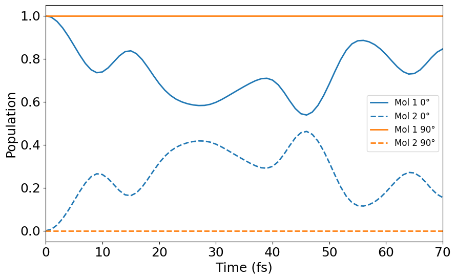
plt.plot(mol1_p[:,0], label="Mol 1 0°", color='tab:blue', linewidth=2)
plt.plot(mol2_p[:,0], label="Mol 2 0°", color='tab:blue', linestyle='--', linewidth=2)
plt.plot(mol1_o[:,0], label="Mol 1 90°", color='tab:orange', linewidth=2)
plt.plot(mol2_o[:,0], label="Mol 2 90°", color='tab:orange', linestyle='--', linewidth=2)
plt.ylabel("Population")
# plt.title("$\Sigma^+$ transition", fontsize=fontsize)
plt.legend(loc='best', fontsize=12)
plt.xlim(0,70)
plt.xlabel("Time (fs)")
[22]:
Text(0.5, 0, 'Time (fs)')
[23]:
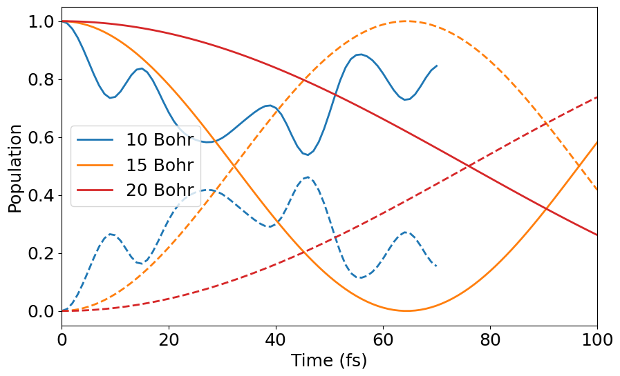
# Now changing the distance between the molecules to 15 and 20 Bohr
data_sigma_plus_para15 = np.loadtxt(f"{path_folder}/pop_15bohr_sigma_plus_para.txt")
data_sigma_plus_para20 = np.loadtxt(f"{path_folder}/pop_20bohr_sigma_plus_para.txt")

mol1_p15 = []
mol2_p15 = []
for i in range(0,len(data_sigma_plus_para15),2):
    mol1_p15.append(data_sigma_plus_para15[i])
for i in range(1,len(data_sigma_plus_para15),2):
    mol2_p15.append(data_sigma_plus_para15[i])
mol1_p15 = np.array(mol1_p15)
mol2_p15 = np.array(mol2_p15)
mol1_p20 = []
mol2_p20 = []
for i in range(0,len(data_sigma_plus_para20),2):
    mol1_p20.append(data_sigma_plus_para20[i])
for i in range(1,len(data_sigma_plus_para20),2):
    mol2_p20.append(data_sigma_plus_para20[i])
mol1_p20 = np.array(mol1_p20)
mol2_p20 = np.array(mol2_p20)
plt.figure(figsize=(10, 6))
plt.plot(mol1_p[:,0], label="10 Bohr", color='tab:blue',lw=2)
plt.plot(mol2_p[:,0], color='tab:blue', linestyle='--', lw=2)
plt.plot(mol1_p15[:,0], label="15 Bohr", color='tab:orange', lw=2)
plt.plot(mol2_p15[:,0], color='tab:orange', linestyle='--', lw=2)
plt.plot(mol1_p20[:,0], label="20 Bohr", color='tab:red', lw=2)
plt.plot(mol2_p20[:,0], color='tab:red', linestyle='--', lw=2)
plt.xlabel("Time (fs)")
plt.ylabel("Population")
plt.xlim(0, 100)
plt.legend()
[23]:
<matplotlib.legend.Legend at 0x15c3522d0>
[24]:
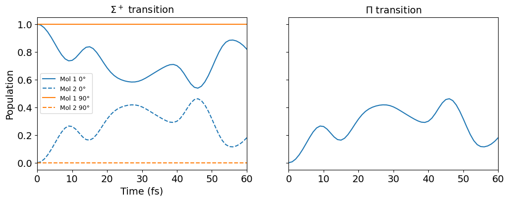
fontsize = 14
plt.rcParams.update({'font.size': fontsize})
#make subplots for each mode
fig, axs = plt.subplots(1, 2, figsize=(12, 4), sharex=True, sharey=True)

axs[0].plot(mol1_p[:,0], label="Mol 1 0°", color='tab:blue')
axs[0].plot(mol2_p[:,0], label="Mol 2 0°", color='tab:blue', linestyle='--')
axs[0].plot(mol1_o[:,0], label="Mol 1 90°", color='tab:orange')
axs[0].plot(mol2_o[:,0], label="Mol 2 90°", color='tab:orange', linestyle='--')
axs[0].set_ylabel("Population")
axs[0].set_title("$\Sigma^+$ transition", fontsize=fontsize)
axs[0].legend(loc='best', fontsize=9)

axs[0].set_xlabel("Time (fs)")
# less spacecing between subplots
axs[1].set_title("$\Pi$ transition", fontsize=fontsize)

axs[1].plot(mol1_p[:,1], label="Mol 1 0°", color='tab:blue')


axs[0].set_xlim(0, 60)
<>:11: SyntaxWarning: invalid escape sequence '\S'
<>:16: SyntaxWarning: invalid escape sequence '\P'
<>:11: SyntaxWarning: invalid escape sequence '\S'
<>:16: SyntaxWarning: invalid escape sequence '\P'
/var/folders/b3/6tj8lwzs2gs_wn_5lp4nnfmw0000gn/T/ipykernel_63422/3761690469.py:11: SyntaxWarning: invalid escape sequence '\S'
  axs[0].set_title("$\Sigma^+$ transition", fontsize=fontsize)
/var/folders/b3/6tj8lwzs2gs_wn_5lp4nnfmw0000gn/T/ipykernel_63422/3761690469.py:16: SyntaxWarning: invalid escape sequence '\P'
  axs[1].set_title("$\Pi$ transition", fontsize=fontsize)
[24]:
(0.0, 60.0)
[25]:
path_new = "../../../paper_pyvcham/dipole_1d"
time= np.loadtxt(f"{path_new}/time.txt")
pop_disp = np.loadtxt(f"{path_new}/pop.txt")
pop_perf = np.loadtxt(f"{path_new}/perfect/pop.txt")

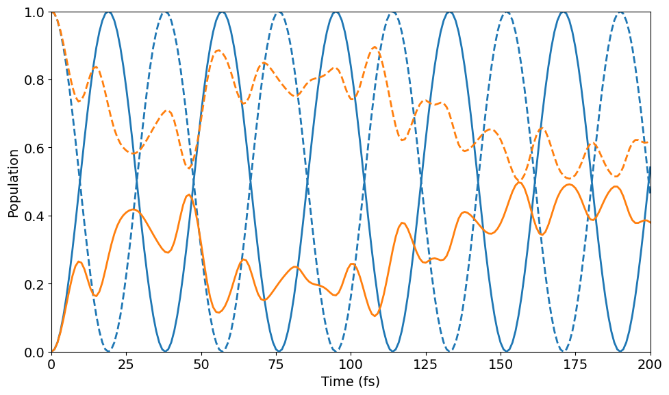
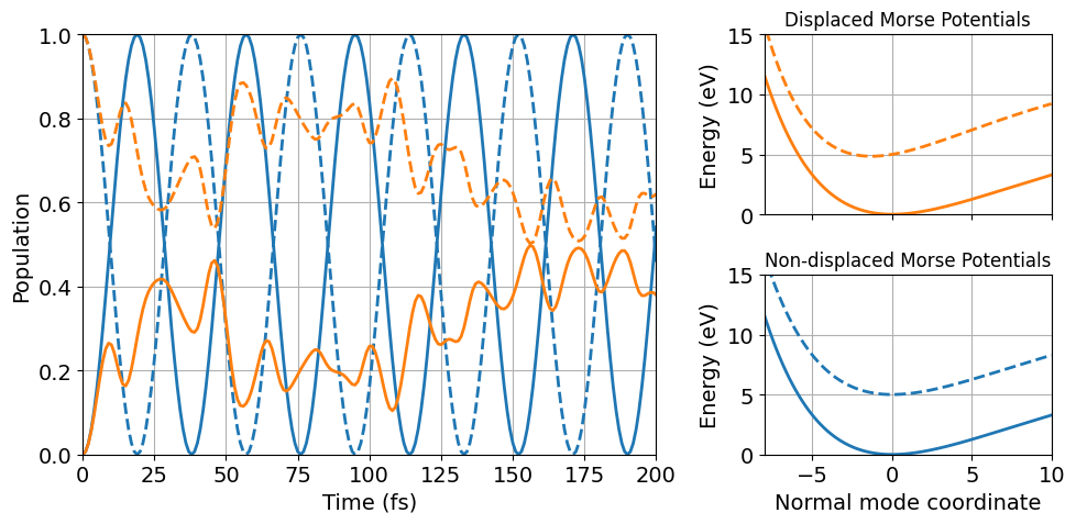
plt.figure(figsize=(10, 6))
plt.plot(time, pop_perf[:,0], color='tab:blue', lw=2)
plt.plot(time, pop_perf[:,1], color='tab:blue', linestyle='--', lw=2)
plt.plot(time, pop_disp[:,0], color='tab:orange', lw=2)
plt.plot(time, pop_disp[:,1], color='tab:orange', linestyle='--', lw=2)
plt.xlim(0, 200)
plt.ylim(0, 1)
plt.xlabel("Time (fs)")
plt.ylabel("Population")
plt.tight_layout()
[26]:
def general_morse(q, params, gs = False):

    De, alpha, q0 = params[0], params[1], params[2]
    if gs:
        q0 = 0.0
    ONE = 1.0
    # Compute the vertical offset at q=0
    offset = De * (np.exp(alpha * q0) - ONE) ** 2
    morse = De * (np.exp(-alpha * (q - q0)) - ONE) ** 2
    return morse - offset

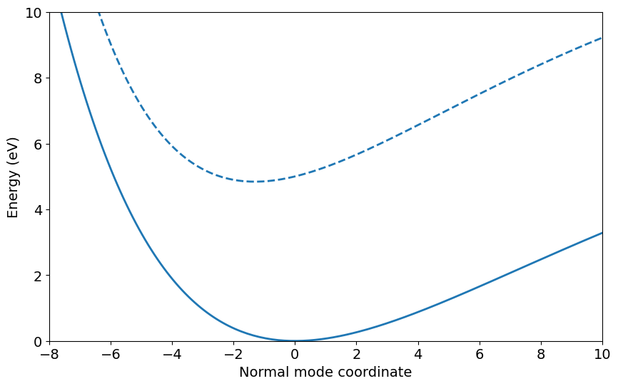
q = np.linspace(-10, 10, 200)
params = [8.613736152648926, 0.09606985002756119, 0.0]
params1 = [8.323473930358887, 0.11420721560716629, -1.304962396621704]
plt.figure(figsize=(10, 6))
plt.plot(q, general_morse(q, params, gs=True), label="GS", color='tab:blue', linewidth=2)
plt.plot(q, general_morse(q, params1, gs=False)+ 5.0 , label="EX1", color='tab:blue', linestyle='dashed', linewidth=2)
# plt.vlines(0, 0, 10, colors='gray', linestyles='solid')
# plt.vlines(-1.304962396621704, 0, 10, colors='gray', linestyles='dashed')
plt.ylim(0, 10)
plt.xlim(-8, 10)
plt.xlabel("Normal mode coordinate")
plt.ylabel("Energy (eV)")
[26]:
Text(0, 0.5, 'Energy (eV)')
[27]:
import matplotlib.pyplot as plt
import numpy as np

# Create figure and GridSpec layout
fig = plt.figure(figsize=(10, 5))
gs = fig.add_gridspec(2, 2, width_ratios=[2, 1], height_ratios=[1, 1])

# Large subplot on the left
ax1 = fig.add_subplot(gs[:, 0])
ax1.plot(time, pop_perf[:,0], color='tab:blue', lw=2)
ax1.plot(time, pop_perf[:,1], color='tab:blue', linestyle='--', lw=2)
ax1.plot(time, pop_disp[:,0], color='tab:orange', lw=2)
ax1.plot(time, pop_disp[:,1], color='tab:orange', linestyle='--', lw=2)
ax1.set_xlim(0, 200)
ax1.set_ylim(0, 1)
ax1.set_xlabel("Time (fs)")
ax1.set_ylabel("Population")

# ax1.legend()
ax1.grid(True)

# Top right subplot
ax2 = fig.add_subplot(gs[0, 1])
ax2.plot(q, general_morse(q, params, gs=True), label="GS", color='tab:orange', linewidth=2)
ax2.plot(q, general_morse(q, params1, gs=False)+ 5.0 , label="ES", color='tab:orange', linestyle='dashed', linewidth=2)
ax2.set_title('Displaced Morse Potentials', fontsize=12)
ax2.set_ylim(0, 15)
ax2.set_xlim(-8, 10)
ax2.set_ylabel('Energy (eV)')

ax2.grid(True)
ax2.set_xticklabels([])  # Hide x-axis labels for top subplot

# Bottom right subplot (shares x-axis with top right)
ax3 = fig.add_subplot(gs[1, 1])#, sharex=ax2)
ax3.plot(q, general_morse(q, params, gs=True), label="GS", color='tab:blue', linewidth=2)
ax3.plot(q, general_morse(q, params, gs=False)+5.0, label="ES", color='tab:blue', linestyle='dashed', linewidth=2)
ax3.set_ylim(0, 15)
ax3.set_xlim(-8, 10)
ax3.set_title('Non-displaced Morse Potentials', fontsize=12)
ax3.set_xlabel('Normal mode coordinate')
ax3.set_ylabel('Energy (eV)')
ax3.grid(True)

# Adjust layout to prevent overlap
plt.tight_layout()
\(\text {FCHO Single molecule}\)
[28]:
# Extracting data from MCTDH calculations for the single molecule and 15 Bohr distance

data_single = np.loadtxt(f"{path_folder}/pop_single.txt")
data_10b = np.loadtxt(f"{path_folder}/pop_15bohr.txt")

mol1_10b =[]
mol2_10b = []
for i in range(0, len(data_10b), 2):
    mol1_10b.append(data_10b[i])
for i in range(1, len(data_10b), 2):
    mol2_10b.append(data_10b[i])
mol1_10b = np.array(mol1_10b)
mol2_10b = np.array(mol2_10b)
[29]:
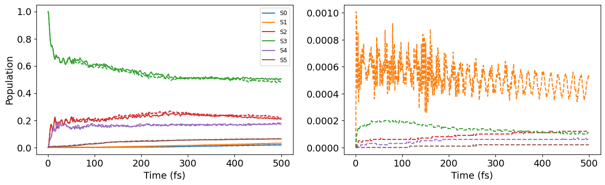
fig, axs = plt.subplots(1, 2, figsize=(15, 4), sharex=True)

# Define the colors for the plots
colors = ['tab:blue', 'tab:orange', 'tab:red', 'tab:green', 'tab:purple', 'tab:brown']
for state in range(6):
    # keep color consistent with previous plots
    axs[0].plot(data_single[:, state], label=f"S{state}", color=colors[state])
    axs[0].plot(mol2_10b[:, state], linestyle='--', color=colors[state], markersize=2)
    if state != 0:
        axs[1].plot(mol1_10b[:, state], label=f"S{state}", linestyle='--', color=colors[state])

axs[0].set_xlabel("Time (fs)")
axs[1].set_xlabel("Time (fs)")
axs[1].set_yticks(np.arange(0, 0.0012, 0.0002))
axs[1].set_yticklabels([f"{x:.4f}" for x in axs[1].get_yticks()])
axs[0].set_ylabel("Population")
axs[0].legend(loc='best', fontsize=9)
[29]:
<matplotlib.legend.Legend at 0x15b7e55e0>